Virtual Imaging#

Place a virtual detector over the diffraction pattern and form a real-space image from what it integrates at every scan position.

Follow along in the app

Every step below is also a live walkthrough inside SpyDE: Help → Virtual Imaging → Guided tour. The tour loads the same small tutorial dataset for you (no download), highlights each control as you go, and closes the example data again when you exit.

Steps#

1. What you’ll do#

A virtual image integrates the diffraction intensity inside a chosen detector region at every scan position, forming a real-space map. Move or resize the detector and the image updates live.

Tip

A small tutorial scan (Tutorial Data → Navigation & Virtual Imaging) is loaded for you — no download needed.

2. Start from a diffraction pattern#

The signal window shows the pattern under the navigator crosshair. Virtual Imaging lives on this window’s toolbar.

$Start from a diffraction pattern$

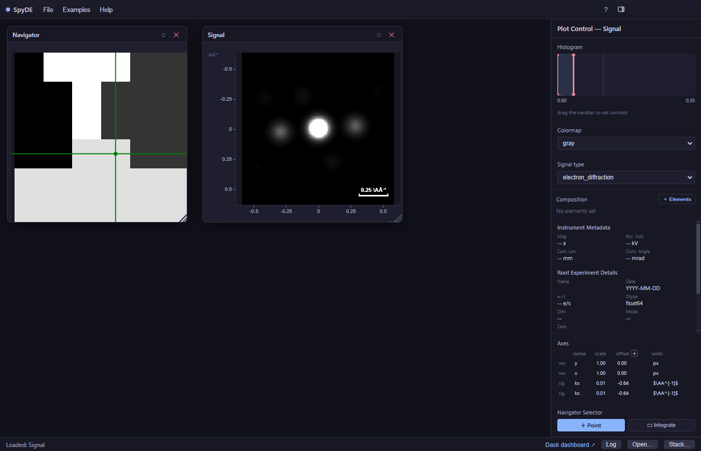
3. Open the Virtual Imaging tools#

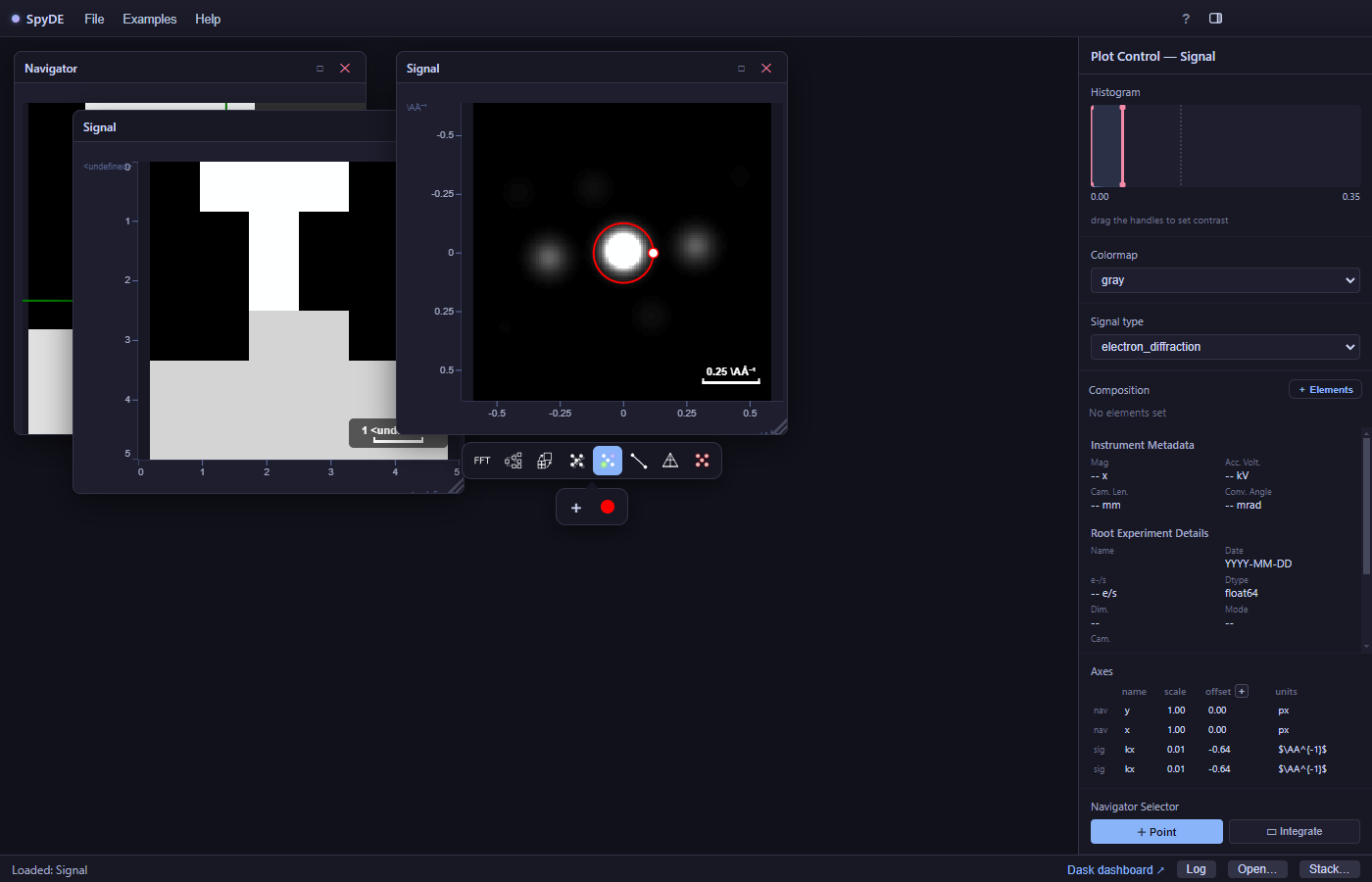
Click Virtual Imaging on the toolbar. A sub-toolbar appears where you add and manage detector regions.

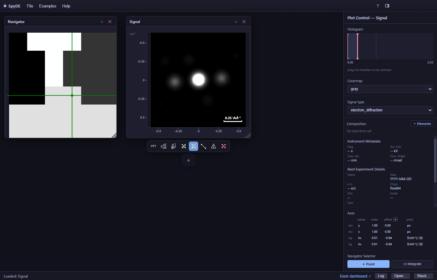
4. Add a detector → a virtual image#

Add a detector region and a virtual image window opens, filled from the intensity it integrates across the scan. Drag or resize the detector on the pattern to update the image live.

Tip

Try it below — drag the green detector over a diffraction spot and watch the scan map light up wherever that spot appears.

More information#

A virtual image is formed after the fact, in software, from a 4D-STEM dataset: you choose a region of the diffraction pattern (a virtual detector) and integrate the intensity inside it at every scan position. Because the choice is made after acquisition, one dataset yields as many images as you want — a small disk on the direct beam gives virtual bright field, an annulus gives virtual annular dark field, and a disk on one Bragg reflection gives a virtual dark-field image showing only the grains that satisfy that reflection.

The detector shape is the experiment. Moving it across the pattern and watching the real-space image change is usually more informative than any single fixed choice, which is why SpyDE recomputes it live as you drag.

Tip

The same operation in a notebook, with pyxem, is linked below.