

Finding Diffraction Vectors#
Detect Bragg peaks across a 4D-STEM scan and overlay the found vectors on the live diffraction pattern.
Follow along in the app
Every step below is also a live walkthrough inside SpyDE: Help → Finding Diffraction Vectors → Guided tour. The tour loads the same small tutorial dataset for you (no download), highlights each control as you go, and closes the example data again when you exit.
Steps#
1. What you’ll do#
Diffraction-vector finding locates the Bragg disks in every diffraction pattern of a 4D-STEM scan. The result is a sparse set of peaks per scan position — the input to virtual imaging, strain, and orientation mapping.
Tip
A small tutorial scan (Tutorial Data → Find Vectors, Si grains) is loaded for you — no download needed.
2. The two linked windows#
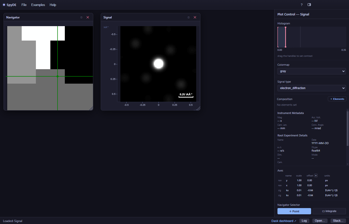
Opening a 4D dataset gives you a navigator (the scan grid) and a signal window (the diffraction pattern at the crosshair). Moving the crosshair on the navigator updates the pattern live.
3. The plot toolbar#
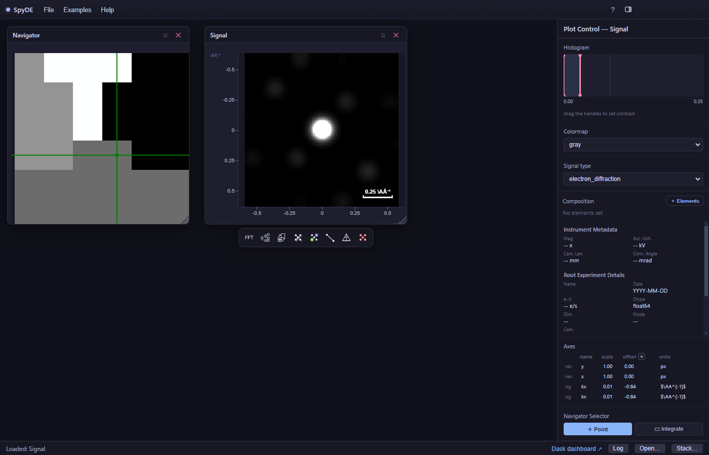
Hover the diffraction-pattern window to reveal its floating toolbar. Tools that act on the signal — FFT, Center Zero Beam, Find Vectors — live here.
4. Open Find Diffraction Vectors#
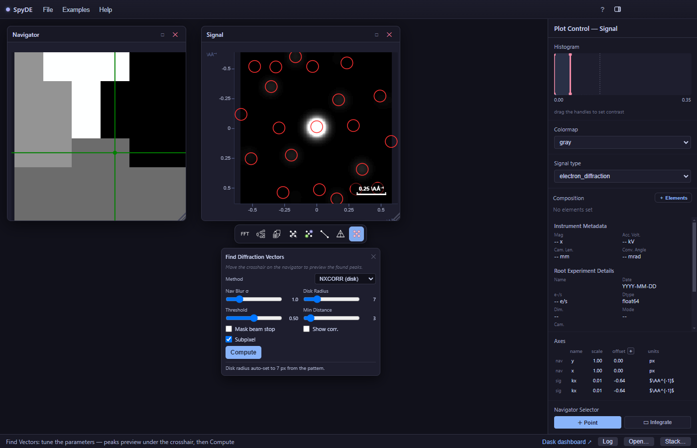
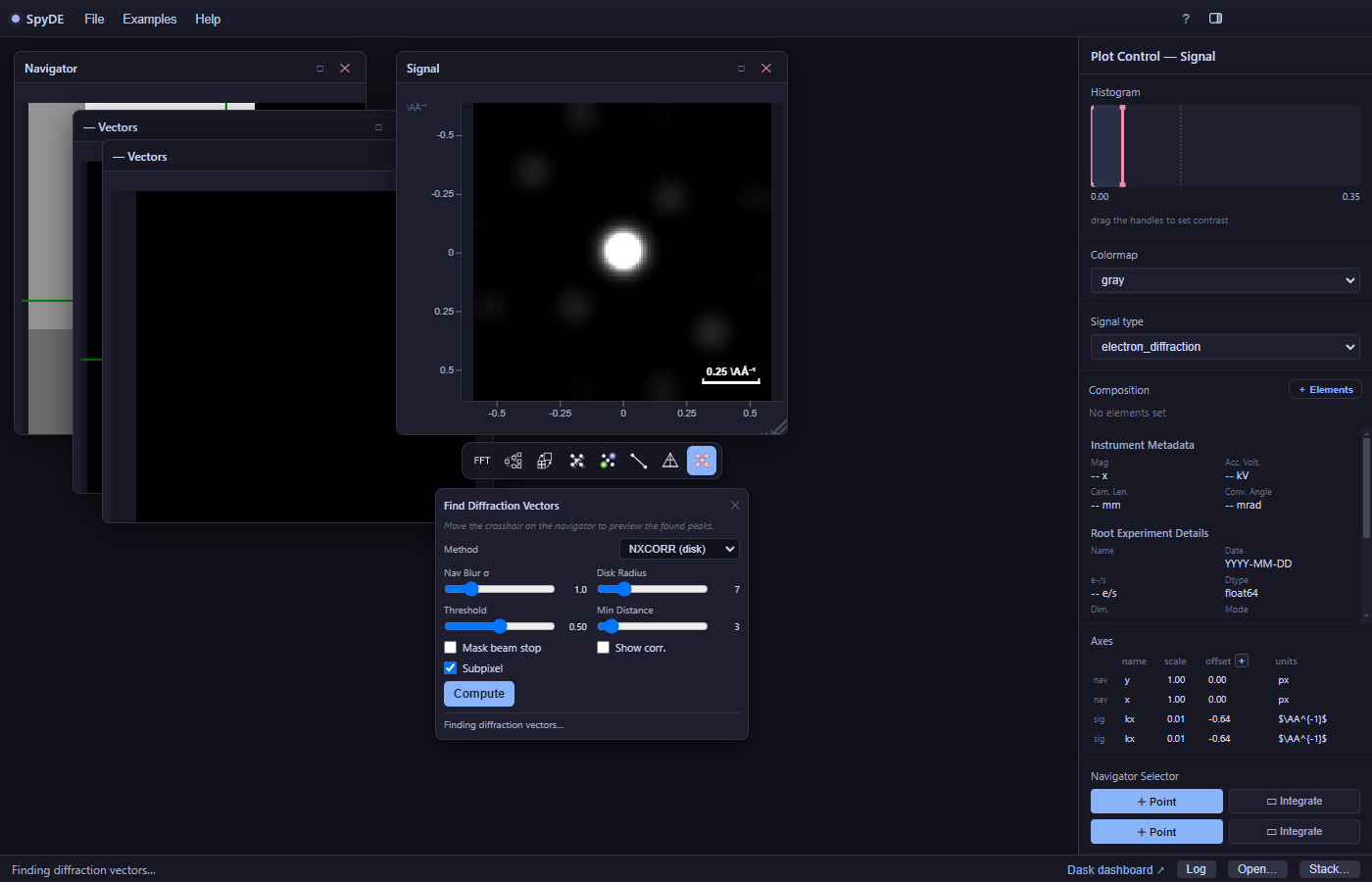
Click the peak-finding tool to open its wizard. It opens with a live preview running on the pattern under the crosshair, so you can tune parameters and see the detected peaks immediately.
5. Tune the detection#
Adjust σ (Gaussian blur before detection) and the threshold (minimum peak strength). Red markers update live on the pattern as you drag the sliders.
Tip
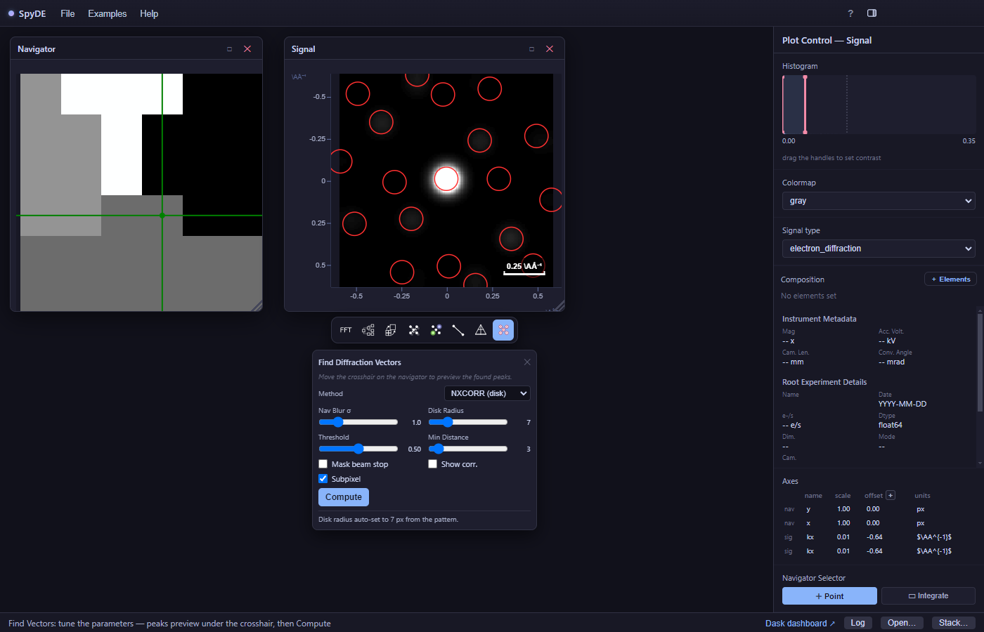
Start with a high threshold and lower it until real disks are marked but noise is not.
6. Compute across the whole scan#
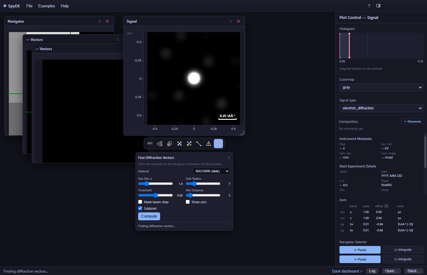
Happy with the preview? Click Compute to run detection on every scan position. Progress streams in the status bar; the found vectors are then overlaid on the live pattern and become a new node in the signal tree.
7. Done — explore the vectors#
When the status bar reports completion, the diffraction vectors are ready. From here you can run Vector Virtual Imaging or Vector Orientation Mapping on them.
Tip
Drag the crosshair across the scan to see each grain’s diffraction pattern with its detected peaks, integrate a region, or virtual-image a single spot.
More information#
Peak (Bragg-disk) finding turns each diffraction pattern into a short list of diffraction vectors — a position in reciprocal space plus an intensity — instead of a dense image. Across a scan that is a ragged, sparse representation of the whole 4D dataset, typically a few hundred times smaller, and it is the input every downstream vector method needs: virtual dark-field imaging, strain from disk positions, and vector-based orientation mapping.
The two knobs that matter are the pre-detection blur σ (suppresses shot noise; too large and neighbouring disks merge) and the threshold (minimum peak strength). Tune them on the live preview of a single pattern before committing to the full scan.
Tip
SpyDE runs the peak finding from pyxem; the pages below are pyxem’s own worked examples of the same operations in a notebook.
Further reading#
SpyDE wraps pyxem, HyperSpy, eXSpy, kikuchipy and orix; those projects document the underlying methods in far more depth than a walkthrough can.
pyxem — Finding diffraction vectors
Template-matching peak finding and subpixel refinement, with the vectors plotted as markers.
-
Window-normalised cross-correlation: how template size and shape change what is detected.
pyxem — Data processing gallery
The wider gallery: centring the zero beam, circular Hough transform, filtering.
pyxem — Working with diffraction vectors
What to do next with a vector set: clustering, unique vectors, sub-pixel positions.